IFRS 9 introduces a new impairment model based on expected credit losses. This is different from IAS 39 Financial Instruments: Recognition and Measurement where an incurred loss model was used.

In accordance with the requirements of IAS 39, impairment losses on financial assets measured at amortised cost were only recognised to the extent that there was objective evidence of impairment. In other words, a loss event needed to occur before an impairment loss could be booked.

IFRS 9 introduces a new impairment model based on expected credit losses, resulting in the recognition of a loss allowance before the credit loss is incurred. Under this approach, entities need to consider current conditions and reasonable and supportable forward-looking information that is available without undue cost or effort when estimating expected credit losses. IFRS 9 sets out a ‘general approach’ to impairment. However, in some cases this ‘general approach’ is overly complicated and some simplifications were introduced.

‘General approach’ to impairment
Under the ‘general approach’, a loss allowance for lifetime expected credit losses is recognised for a financial instrument if there has been a significant increase in credit risk (measured using the lifetime probability of default) since initial recognition of the financial asset. If, at the reporting date, the credit risk on a financial instrument has not increased significantly since initial recognition, a loss allowance for 12-month expected credit losses is recognised. In other words, the ‘general approach’ has two bases on which to measure expected credit losses; 12-month expected credit losses and lifetime expected credit losses.

Lifetime expected credit loss is the expected credit losses that result from all possible default events over the expected life of a financial instrument. 12-month expected credit loss is the portion of the lifetime expected credit losses that represent the expected credit losses that result from default events on a financial instrument that are possible within the 12 months after the reporting date.

The term ‘default’ is not defined in IFRS 9 and an entity will have to establish its own policy for what it considers a default, and apply a definition consistent with that used for internal credit risk management purposes for the relevant financial instrument. IFRS 9 includes a rebuttable presumption that a default does not occur later than when a financial asset is 90 days past due unless an entity has reasonable and supportable information to demonstrate that a more lagging default criterion is more appropriate. When it comes to the actual measurement under the ‘general approach’ an entity should measure expected credit losses of a financial instrument in a way that reflects the principles of measurement set out in IFRS 9.

These dictate that the estimate of expected credit losses should reflect:

• an unbiased and probability-weighted amount that is determined by evaluating a range of possible outcomes;
• the time value of money; and
• reasonable and supportable information about past events, current conditions and forecasts of future economic conditions that is available without undue cost or effort at the reporting date.

Putting the theory into practice, expected credit losses under the ‘general approach’ can best be described using the following formula: Probability of Default (PD) x Loss given Default (LGD) x Exposure at Default (EAD). For each forward looking scenario an entity will effectively develop an expected credit loss using this formula and probability weigh the outcomes.

‘Simplified approach’ to impairment
IFRS 9 allows entities to apply a ‘simplified approach’ for trade receivables, contract assets and lease receivables. The simplified approach allows entities to recognise lifetime expected losses on all these assets without the need to identify significant increases in credit risk. Certain accounting policy choices apply:

• For trade receivables and contract assets that do not contain a significant financing component, it is a requirement to recognise a lifetime expected loss allowance (i.e. an entity must always apply the ‘simplified approach’).
• For other trade receivables, other contract assets, operating lease receivables and finance lease receivables it is an accounting policy choice that can be separately applied for each type of asset (but which applies to all assets of a particular type).

A significant financing component exists if the timing of payments agreed to by the parties to the contract (either explicitly or implicitly) provides the customer or the entity with a significant benefit of financing the transfer of goods or services to the customer. [IFRS 15:60]

Applying the ‘simplified approach’ using a provision matrix
When applying the ‘simplified approach’ to, for example, trade receivables with no significant financing component, a provision matrix can be applied. A provision matrix is nothing more than applying the relevant loss rates to the trade receivable balances outstanding (i.e. a trade receivable aged analysis). Because IFRS 9 does not provide any specific guidance on this issue, we provide a stepped approach to using a provision matrix below.

Step 1 Determine the appropriate groupings of receivables
There is no explicit guidance or specific requirement in IFRS 9 on how to group trade receivables, however, groupings could be based on geographical region, product type, customer rating, collateral or trade credit insurance and type of customer (such as wholesale or retail).

To be able to apply a provision matrix to trade receivables, the population of individual trade receivables should first be aggregated into groups of receivables that share similar credit risk characteristics. When grouping items for the purposes of shared credit characteristics, it is important to understand and identify what most significantly drives each different group’s credit risk.

Step 2 Determine the period over which historical loss rates are appropriate
Once the sub-groups are identified, historical loss data need to be collected for each sub-group. There is no specific guidance in IFRS 9 on how far back the historical data should be collected. Judgment is needed to determine the period over which reliable historical data can be obtained that is relevant to the future period over which the trade receivables will be collected. In general, the period should be reasonable – not an unrealistically short or long period of time. In practice, the period could span two to five years.

Step 3 Determine the historical loss rates
Now that sub-groups have been identified and the period over which loss data will be captured has been selected, an entity determines the expected loss rates for each sub-group sub-divided into past-due categories. (i.e. a loss rate for balances that are 0 days past due, a loss rate for 1-30 days past due, a loss rate for 31-60 days past due and so on). To do so, entities should determine the historical loss rates of each group or sub-group by obtaining observable data from the determined period.

IFRS 9 does not provide any specific guidance on how to calculate loss rates and judgement will be required.

Step 4 Consider forward looking macro-economic factors and conclude on appropriate loss rates
The historical loss rates calculated in Step 3 reflect the economic conditions in place during the period to which the historical data relate. While they are a starting point for identifying expected losses they are not necessarily the final loss rates that should be applied to the carrying amount. It should be determined whether the historical loss rates were incurred under economic conditions that are representative of those expected to exist during the exposure period for the portfolio at the balance sheet date.

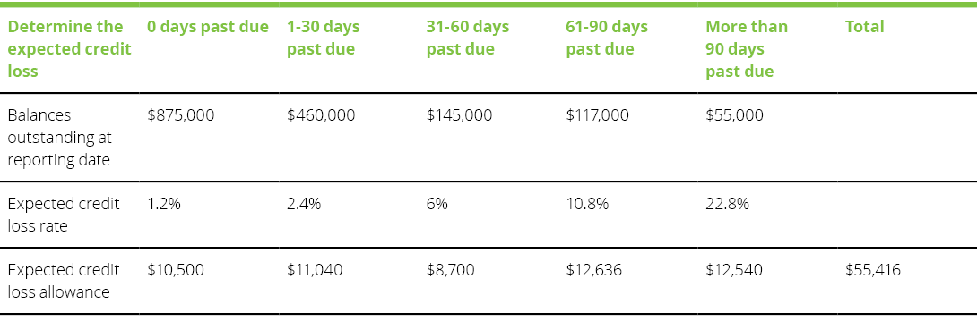
Step 5 Calculate the expected credit losses
The expected credit loss of each sub-group determined in Step 1 should be calculated by multiplying the current gross receivable balance by the loss rate. For example, the specific adjusted loss rate should be applied to the balance of each age-band for the receivables in each group. Once the expected credit losses of each age-band for the receivables have been calculated, then simply add all the expected credit losses of each age-band for the total expected credit loss of the portfolio. The table below illustrates how the ultimate expected credit loss allowance would be calculated using the loss rates calculated in Step 4.

More information about applying the provision matrix approach in practice, including a detailed illustrative example, can be found in the publication issued by Deloitte Global Office which is available here.

Source: A Closer Look — Applying the expected credit loss model to trade receivables using a provision matrix

The article is part od dReport – November 2018, Accounting news.